I was teaching Ohms laws law and introductory circuit calculations bout two days ago at a Swedish gymnasium, a subject which I’m about as adept as now as I was when I myself took the class 7 or so years ago. There are basically only two formulas one has to learn in that course and those are the two effective resistance formulas for resistors in series and resistors in paralell

Not sufficient to describe circuits with more complicated typologies such as bridges like the Wheatstone bridge but sufficient for at least engaging in some basic design.
The problem which came to mind as I was reviewing the material was how one would set out to build a circuit element with a specified resistance from a given set of elements. Usually it’s the other way around. You get the component and you compute the resistance but the inverse problem of getting a specified resistance and then designing the circuit from some pieces if of course a lot more interesting and as we shall see in this special case surprisingly straightforward.
Let us study this particular problem: “Given a set of resistors with resistance  how does one combine these to form an element with a specified fractional resistance
  “. If we want an integer multiple or integer fraction or a specific resistance then things are straightforward, just chain
  together to get a resistance
  or put
  in parallell to
  and this is the smallest number of equal number of components you need.
For fractional resistances of a more general form however there are clearly very different ways you can go about designing the circuit and there are different benefits to them
Solution one: Construct $latex $q$ chains with resistors each and put those chains in parallel
m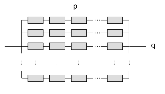 The chains have resistance
  and putting $latex $q$ of them in paralell reduces the total resistance by a th to
  .
.
Solution two: Another is to first create blocks of $latex $ resistors in paralell and then put those in series. However both of these solution has the disadvantage that it requires a total number of
  resistors to complete it which for most fractions becomes very impractical.
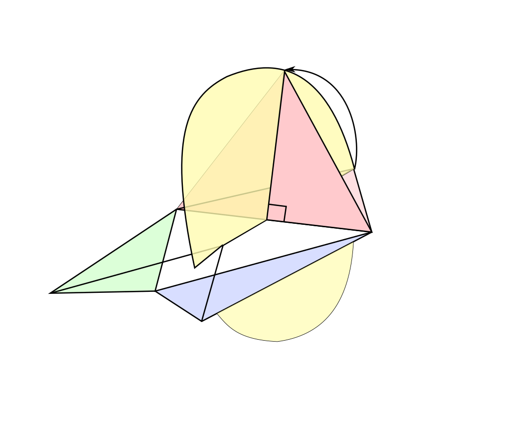
My question was therefore if there was a simple way to get a component with this resistance but which wouldn’t require quite so many resistors. Let us just start off by making clear that it is possible. These two components you see below both have the same resistance 

but the right one was built using only 3 resistors instead of 6 which is (if you count by means of manufacturing cost) is a more effective solution. And the process or computing the resistance of the latter composition betrays the coming idea

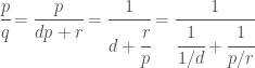
(I will henceforth just set  ) Usually one would have used ^(-1)-notation for the parallell coupling but not doing that reveals the continued fraction expression associated with this construction.
The central idea can be laid out as follows inductively. If you want to design a component with resistance $p/q$ (where  is a reduced fraction such that
  ) perform euclidean division and rearrange it according to
1
We now recognize the right hand side as the expression for the resistance of two resistor with resistance  and
and  in parallel. The idea can diagrammaticaly be represented by

The resistor is constructed by putting  resistors in parallel and the resistor is constructed by repeating the induction step.**
This can be streamlined by first computing the continued fraction of a fraction and then move backwards to form these construction steps . Take for example the continued fraction for 
![\cfrac{7}{24} = \cfrac{1}{3 + \cfrac{1}{2 + \cfrac{1}{3}}}= [0; 3,2,3]](https://s0.wp.com/latex.php?latex=%5Ccfrac%7B7%7D%7B24%7D+%3D+%5Ccfrac%7B1%7D%7B3+%2B+%5Ccfrac%7B1%7D%7B2+%2B+%5Ccfrac%7B1%7D%7B3%7D%7D%7D%3D+%5B0%3B+3%2C2%2C3%5D&bg=ffffff&fg=444444&s=0&c=20201002)
which now contains a recipe for designing the composite resistor

Where the top 3-parallell component corresponds to [0;3,2,3], the 2-series at the bottom to [0;3,2,3], and the 3 in series at the bottom to [0;3,2,3].
Not all continued fractions will however have so small numbers in the expansion and especially when the numerator and denominator are fibonnacci numbers we’ll still end up with having to use a very large number of resistors.
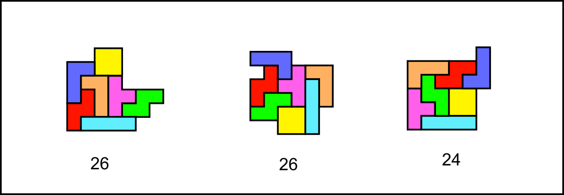
What is kind of nice though is that irrational numbers which have a quickly convergent continued fraction can be approximated pretty accurately.  for example has a continued fraction [3;7,15,1,292,1,1,…] which means you can use the approximation
 ![\pi \approx [3;7,15,1] = [3;7,16]](https://s0.wp.com/latex.php?latex=%5Cpi+%5Capprox+%5B3%3B7%2C15%2C1%5D+%3D+%5B3%3B7%2C16%5D&bg=ffffff&fg=444444&s=0&c=20201002) which using only 26 resistors gives 6 digits of pi which is pretty neat. A
which using only 26 resistors gives 6 digits of pi which is pretty neat. A

I’ve got half a mind to build this circuit to see if it checks out but unfortunately cheap hobby resistors only have about 1% accuracy to them so you’d only really end up with 3 digits tops.
EDIT: Many of the diagrams in the original publications had errors in them which made them not agree with the text and which were corrected around one hour later.


has no real solutions and since the polynomial has real coefficients the 4 non-real solutions come in conjugate pairs.


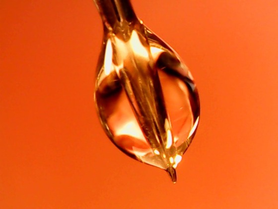
 In my home when I grew up there used to hang a weird glass fixture above the stair leading to the basement. It was always half full with water but I never really paid it much attention. At some point I asked what it was for and got some cryptic answer from my mom that it was for predicting whether it would rain. Ignoring something which was obviously magic I never did figure out how it worked until much later learning about mercury barometers in high school at least the principle became clear.

 (The volume of the liquid is constant)
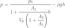
 (Ideal gas law)
 (Pascals law)
 . From the geometric constraints we get

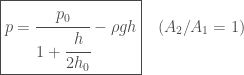
 so in the grand scheme of things it can be neglected which besides implying
  and
and  also simplifies the expression
 is the same order of magnitude as
  in which case the trapped gas volume would remain close to original pressure.

 Didaktik (Mathematics for teachers), page 270 we find a suggested seminar acticity which mentions the following (meta problem).
 and
and 
 by essentially explaining the pattern
 implies a = 0 or b = 0, and solve some quadratics that have already been factored like
  .
. by factoring
  and then applying the ZPP.
 . (This does not use the ZPP nor the conjugate rule)


 (This should be complemented by graphing)
 by factoring with the difference of squares and applying the zero product rule.
  and
and  and sneaking in problems the type
 by factoring with the distributive property

 )
) ,which is why it’s probably not used but it would be interesting to try it (or hear about if these is a book or school system) which approaches it this way. The final step 6, the method of factoring a general quadratic directly with the difference of squares is a technique which I find would be a useful addition to the scheme as I think it neatly exposes the connection between the three different forms in which you can write a quadratic expression in an algorithmic way instead of in a more formally logical way (invoking the general factor theorem).


 .
. . Applying the Euclidean algorithm we have

 and we summarize
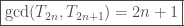
 Applying the Euclidean algorithm again we have


 .
.
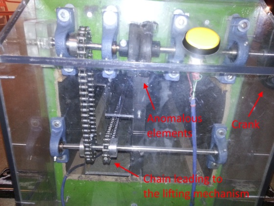
 and here slightly more magnified.